○Draft — not verified

Top-down comparison of four wheel configurations: differential drive, Ackermann, omnidirectional, and tracked — Four drive configurations compared top-down — differential, Ackermann, omnidirectional, and tracked — with their holonomic vs. nonholonomic character called out.

Theoretical Background: Mobile Robotic Systems

Module 1 Theory: Introduction to Mobile Robotic Systems

1.3.1 Components of Mobile Robots

A mobile robot is a self-contained electromechanical system capable of navigating through its environment. Understanding the physical and computational subsystems that make up a mobile robot is essential before studying its kinematics or control. Every mobile robot, regardless of its application, consists of a mechanical platform, actuation, power, sensing, and computation.

Chassis and Mechanical Platform

The chassis is the structural frame that supports all other components. In mobile robotics, the chassis defines the robot’s footprint, weight distribution, and mounting points for sensors and actuators. Materials range from aluminum extrusions in research platforms to injection-molded plastics in consumer robots. The chassis geometry directly affects stability, which depends on the relationship between the center of gravity and the support polygon formed by the wheel contact points.

Actuators

Actuators convert electrical energy into mechanical motion. The three dominant actuator types in mobile robotics are:

DC Motors: Provide continuous rotation with speed proportional to applied voltage. Brushed DC motors are inexpensive and easy to control but suffer from brush wear. Brushless DC (BLDC) motors eliminate this issue at the cost of more complex drive electronics. DC motors are the standard choice for driving wheels in differential drive robots.
Servo Motors: Integrate a DC motor with a position feedback sensor (typically a potentiometer or encoder) and a control circuit. Standard hobby servos provide position control over a limited range (0-180 degrees), while continuous rotation servos behave like speed-controlled DC motors. Servos are commonly used for steering mechanisms and sensor pan-tilt units.
Stepper Motors: Rotate in discrete angular increments (steps), typically 1.8 degrees per step. They provide precise open-loop position control without requiring feedback sensors. However, stepper motors have lower power density than DC motors and can miss steps under high load. They are used in applications requiring precise angular positioning, such as LiDAR rotation stages.

Power Systems

Mobile robots are untethered and must carry their own energy source. Lithium polymer (LiPo) batteries dominate due to their high energy density, typically providing 150-200 Wh/kg. Power management involves voltage regulation (motors, sensors, and processors often require different voltages), current limiting to protect electronics, and battery monitoring to prevent over-discharge. The battery capacity directly constrains the robot’s operational duration, making power efficiency a first-order design concern.

Sensors

Sensors provide the robot with information about itself and its environment. They are classified into two categories based on what they measure:

Proprioceptive Sensors measure the robot’s internal state. Wheel encoders measure rotation and provide odometry estimates. Inertial measurement units (IMUs) contain accelerometers and gyroscopes that measure linear acceleration and angular velocity. Battery voltage sensors monitor power state. These sensors answer the question: what is the robot doing?
Exteroceptive Sensors measure the external environment. LiDAR provides 2D or 3D distance measurements by emitting laser pulses and measuring return time. Cameras provide rich visual information for object detection, visual odometry, and SLAM. Ultrasonic sensors measure distance using sound pulses. Infrared sensors detect proximity at short range. Bumper switches detect physical contact. These sensors answer the question: what is around the robot?

Key Distinction: Proprioceptive sensors accumulate drift over time because they integrate measurements. Exteroceptive sensors provide absolute measurements relative to the environment but are subject to noise, occlusion, and varying environmental conditions.

Computing Hardware

The onboard computer runs perception, planning, and control algorithms. Common platforms include single-board computers (Raspberry Pi, NVIDIA Jetson) for mid-level computation, microcontrollers (Arduino, STM32) for real-time low-level motor control, and GPU-equipped boards for deep learning inference. Many robots use a heterogeneous architecture where a microcontroller handles motor control at high frequency (1 kHz+) while a Linux-based computer handles perception and planning at lower frequency (10-30 Hz).

1.3.2 Sensing, Planning, and Actuation Pipeline

The Sense-Plan-Act Paradigm

The classical architecture for autonomous mobile robots follows a three-stage pipeline: sense the environment, plan a course of action, and execute that plan through actuators. This paradigm, while simplified, provides a useful framework for understanding how information flows through a robotic system.

Perception is the process of interpreting raw sensor data into meaningful representations of the world. A LiDAR scan returns thousands of distance measurements, but the robot needs to identify walls, obstacles, and open spaces. Perception algorithms include obstacle detection, object recognition, terrain classification, and feature extraction. The output of perception feeds into the robot’s internal world model.

Localization answers the question: where am I? The robot must determine its position and orientation within a known or partially known environment. Odometry provides a local estimate by integrating wheel encoder data, but this drifts over time. More robust methods fuse odometry with exteroceptive sensor data. The extended Kalman filter and particle filter are standard approaches for combining multiple noisy sensor measurements into a coherent state estimate.

Mapping answers the question: what does the world look like? When the environment is unknown, the robot must construct a map from sensor observations while simultaneously localizing within that map. This chicken-and-egg problem is known as Simultaneous Localization and Mapping (SLAM) and is one of the fundamental challenges in mobile robotics. Occupancy grid maps discretize the environment into cells labeled as free, occupied, or unknown.

Path Planning computes a collision-free route from the robot’s current position to a goal. Global planners (A*, Dijkstra, RRT) find paths through the known map. Local planners (DWA, TEB) generate short-horizon trajectories that avoid dynamic obstacles and respect the robot’s kinematic constraints. The distinction between global and local planning allows the robot to follow a general route while reacting to unexpected obstacles.

Motion Control translates planned trajectories into actuator commands. A trajectory tracking controller computes the linear and angular velocities needed to follow the planned path, then converts these into individual wheel speeds. PID controllers are the standard approach for regulating wheel velocity to match the commanded setpoint.

1.3.3 Locomotion Mechanisms

The choice of locomotion mechanism fundamentally determines a mobile robot’s kinematic model, maneuverability, terrain capability, and control complexity.

Wheel Arrangements

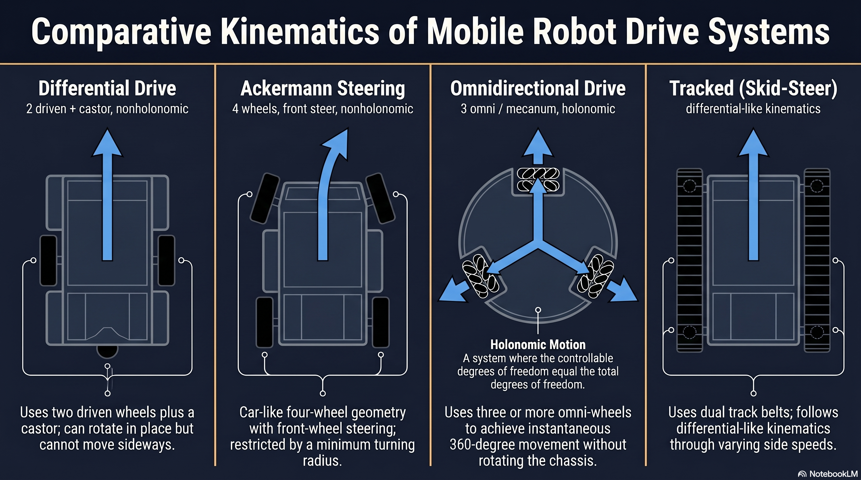
Differential Drive is the most common configuration for indoor mobile robots. Two independently driven wheels are mounted on a common axis, with one or more passive caster wheels for stability. The robot steers by varying the relative speed of the two drive wheels. Equal speeds produce straight-line motion; opposite speeds produce rotation in place. This simplicity of control, combined with the ability to rotate in place (zero-radius turning), makes differential drive the dominant choice for indoor applications. Examples include the TurtleBot, Roomba, and most research platforms.

Omnidirectional Drive uses three or more specially designed wheels (Mecanum or Swedish wheels) that allow the robot to move in any direction instantaneously, including sideways. Mecanum wheels have angled rollers mounted around the wheel circumference, creating force components perpendicular to the wheel axis. A typical configuration uses four Mecanum wheels arranged in a rectangle. While omnidirectional drive eliminates steering constraints, it reduces traction and payload capacity due to the roller contact geometry. It is used in warehouse logistics (KUKA youBot) and robotic soccer.

Ackermann Steering follows the geometry of conventional automobiles, where front wheels pivot about different centers to maintain a common instantaneous center of rotation. This prevents tire scrubbing during turns. The turning radius is bounded below by the mechanical steering limits, meaning the robot cannot rotate in place. Ackermann steering is the standard for outdoor autonomous vehicles because it provides stable high-speed turning with predictable dynamics.

Drive Mechanisms

The drive mechanism couples the motor output to the wheels. Direct drive mounts the motor shaft directly to the wheel hub, offering simplicity but requiring low-speed, high-torque motors. Geared drive uses a reduction gearbox to convert high-speed motor rotation into low-speed, high-torque wheel rotation. Belt and chain drives provide flexible coupling between motors and wheels. The gear ratio determines the trade-off between maximum speed and maximum torque.

Steering Mechanisms

In differential drive, steering is achieved through speed difference between left and right wheels — there is no separate steering mechanism. In Ackermann steering, a mechanical linkage connects the steering actuator to the front wheel assemblies, maintaining the correct angular relationship between inner and outer wheels. In omnidirectional systems, steering is achieved through the vector sum of individual wheel forces, with no mechanical steering components at all.

1.3.4 Differential Drive Kinematics

The differential drive robot is the reference platform for this course, and its kinematic model is the foundation for all subsequent motion planning and control work.

Forward Kinematics

Given the velocities of the right wheel $v_{R}$ and left wheel $v_{L}$ , the linear velocity v and angular velocity omega of the robot center are:

v = (v_{R} + v_{L}) /2 (1)

ω = (v_{R} - v_{L}) / L (2)

where L is the distance between the two drive wheels (the wheel base or track width). Equation (1) computes the average forward speed, and equation (2) computes the rate of rotation. When $v_{R}$ = $v_{L}$ , the robot moves straight (omega = 0). When $v_{R}$ = - $v_{L}$ , the robot rotates in place (v = 0).

The robot’s pose in the global frame is described by (x, y, theta), where (x, y) is the position of the midpoint between the drive wheels and theta is the heading angle measured from the positive x-axis. The pose evolves according to:

\overset{x}{˙} = v cos (θ) (3)

\overset{y}{˙} = v sin (θ) (4)

\dot{θ} = ω (5)

Equations (3)-(5) constitute the kinematic model of the differential drive robot. This is a system of first-order ordinary differential equations that, given initial conditions ( $x_{0}$ , $y_{0}$ , $θ_{0}$ ) and velocity inputs (v, omega), fully determines the robot’s trajectory over time.

Inverse Kinematics

Given desired robot velocities (v, omega), the required angular velocities of the left and right wheels are:

ω_{L} = \frac{2 v - ω L}{2 r} (6)

ω_{R} = \frac{2 v + ω L}{2 r} (7)

where r is the wheel radius. These equations are derived by solving equations (1) and (2) simultaneously for $v_{L}$ = r $ω_{L}$ and $v_{R}$ = r $ω_{R}$ . Inverse kinematics is used directly in the motor control loop: the high-level planner outputs (v, omega), and equations (6)-(7) convert these into wheel speed commands.

Odometry

By integrating the kinematic equations over discrete time steps, the robot can estimate its pose from wheel encoder measurements alone. Given encoder counts, the wheel displacements Delta_ $s_{R}$ and Delta_ $s_{L}$ over one time step yield:

Δ_{s} Δ_{θ} x_{new} y_{new} θ_{new} = (Δ_{s_{R}} + Δ_{s_{L}}) /2 = (Δ_{s_{R}} - Δ_{s_{L}}) / L = x_{old} + Δ_{s} cos (θ_{old} + \frac{Δ _{θ}}{2}) = y_{old} + Δ_{s} sin (θ_{old} + \frac{Δ _{θ}}{2}) = θ_{old} + Δ_{θ}

This dead-reckoning estimate drifts over time due to wheel slip, uneven surfaces, and encoder quantization errors. The drift rate is typically 1-5% of distance traveled, making odometry useful for short-range motion but unreliable for long-range navigation without correction from exteroceptive sensors.

1.3.5 Holonomic vs. Non-Holonomic Constraints

A constraint is holonomic if it can be expressed purely in terms of position variables: f(q) = 0. A holonomic constraint reduces the dimension of the configuration space. A system with n generalized coordinates and k holonomic constraints has (n - k) degrees of freedom.

A constraint is non-holonomic if it involves velocities and cannot be integrated into a position-only equation. Non-holonomic constraints restrict the instantaneous velocities available to the system but do not reduce the dimension of the configuration space. The system can still reach any configuration, but not through arbitrary paths.

Why Differential Drive is Non-Holonomic

The differential drive robot has a three-dimensional configuration space (x, y, theta) but only two control inputs (v, omega). The constraint that prevents the robot from moving sideways is:

\overset{x}{˙} sin (θ) - \overset{y}{˙} cos (θ) = 0

This equation involves velocities and cannot be integrated to a position constraint. The robot cannot instantaneously slide sideways (perpendicular to its heading), yet it can reach any (x, y, theta) configuration through a sequence of forward motions and rotations. The configuration space is fully reachable, but the velocity space is restricted at every instant.

Key Implication: Non-holonomic constraints make path planning more complex because not every geometric path is kinematically feasible. A straight diagonal line may be geometrically short, but a differential drive robot must execute a sequence of turns and straight segments to follow it. Path planners for non-holonomic systems must generate trajectories that respect the velocity constraints at every point.

Holonomic Systems

An omnidirectional robot with Mecanum wheels is holonomic: it has three degrees of freedom (x, y, theta) and three independent control inputs. It can move in any direction instantaneously without first rotating, making path planning geometrically simpler. The trade-off is increased mechanical complexity and reduced traction.

1.3.6 Instantaneous Center of Rotation (ICR)

At any instant, the motion of a rigid body in the plane can be described as a pure rotation about a single point called the Instantaneous Center of Rotation (ICR). For a differential drive robot, the ICR lies along the line connecting the two drive wheels, at a distance R from the robot center:

R = v / ω = L (v_{R} + v_{L}) / (2 (v_{R} - v_{L}))

Special Cases:

Straight-line motion ( $v_{R}$ = $v_{L}$ ): R approaches infinity — the ICR is at infinity, and the robot moves in a straight line. There is no rotation.
Pure rotation ( $v_{R}$ = - $v_{L}$ ): R = 0 — the ICR is at the midpoint between the wheels. The robot spins in place.
Gentle curve ( $v_{R}$ close to $v_{L}$ ): R is large — the robot follows a wide arc.
Tight curve ( $v_{R}$ much greater than $v_{L}$ ): R is small — the robot follows a tight arc near the slower wheel.
Pivot turn ( $v_{L}$ = 0): R = L/2 — the ICR is at the left wheel. The robot pivots about the stationary wheel.

The ICR concept provides geometric intuition for how differential drive steering works. Every motion of the robot, no matter how complex, can be decomposed into a sequence of circular arcs (or straight lines as a degenerate case) defined by the ICR position at each instant. This geometric understanding is useful when designing trajectory controllers and analyzing motion constraints.

1.3.7 Performance Considerations

Stability

A mobile robot is statically stable if the vertical projection of its center of gravity falls within the support polygon. For a three-wheeled differential drive robot (two drive wheels plus one caster), the support polygon is a triangle. Adding a fourth wheel (second caster) increases the support polygon to a quadrilateral, improving stability at the cost of requiring a suspension or compliant wheel mounting to maintain ground contact on uneven surfaces. Dynamic stability considers the effects of acceleration and deceleration on tipping, which becomes relevant for tall robots or those carrying heavy payloads at height.

Maneuverability

The degree of maneuverability describes how freely a robot can move in its environment. Differential drive provides two controllable DOF (forward motion and rotation) with zero-radius turning capability, making it highly maneuverable in tight spaces. Ackermann steering has a minimum turning radius, reducing maneuverability in confined environments. Omnidirectional drive provides the maximum maneuverability with three independently controllable DOF.

Efficiency

Energy efficiency depends on the locomotion mechanism, terrain, and payload. Wheeled robots on hard, flat surfaces are highly efficient because rolling resistance is low. Tracked robots sacrifice efficiency due to the continuous sliding of track segments. The gear ratio between motor and wheel affects whether the drive system is optimized for speed (high gear ratio) or torque (low gear ratio). Regenerative braking can recover energy during deceleration but adds complexity to the power electronics.

Payload Capacity

The maximum payload is constrained by motor torque, structural strength of the chassis, and stability margins. Increasing payload raises the center of gravity, reduces acceleration capability, and increases stopping distance. The drive motors must be sized to handle the worst-case combined load of the robot’s own weight plus maximum payload on the steepest expected incline.

Integration: Theory to Practice

The component and kinematic models developed in this module map directly to the software architecture of a ROS 2 mobile robot. The kinematic model (equations 1-7) is implemented in the motor controller node, which subscribes to /cmd_vel (receiving v and omega as a geometry_msgs/Twist message) and converts these to wheel speed commands using the inverse kinematics. Wheel encoders feed data into the odometry node, which integrates the forward kinematics to publish pose estimates on /odom as a nav_msgs/Odometry message. Each sensor type corresponds to a ROS 2 driver node that publishes on a standard topic: LiDAR on /scan (sensor_msgs/LaserScan), IMU on /imu (sensor_msgs/Imu), and cameras on /image_raw (sensor_msgs/Image). The tf2 library manages the coordinate frame relationships between the robot base, sensor frames, odometry frame, and map frame. This standardized interface means that the same planning and control algorithms work across different hardware platforms, because the kinematic model is abstracted behind the /cmd_vel and /odom topics.

Theoretical Design Choices

Why differential drive dominates indoor mobile robotics: Differential drive provides the simplest kinematic model that still allows full planar reachability (any pose can be achieved). The two-parameter control input (v, omega) maps naturally to the publish/subscribe architecture used in ROS 2. Zero-radius turning is critical for navigating narrow corridors and doorways in indoor environments. The mechanical simplicity of two driven wheels plus casters minimizes cost, weight, and failure modes. Omnidirectional drive offers greater instantaneous mobility but introduces mechanical complexity (Mecanum wheels, precise roller alignment) and reduces traction, which limits payload. Ackermann steering cannot rotate in place, making it unsuitable for confined indoor spaces. For the vast majority of indoor mobile robotics applications — warehousing, delivery, service, and research — differential drive provides the optimal balance of simplicity, capability, and reliability.

Why non-holonomic constraints matter for planning: The inability of a differential drive robot to move sideways means that geometric shortest paths are generally not kinematically feasible. A path planner that ignores the non-holonomic constraint will generate paths the robot cannot follow. This is why mobile robot path planners (such as the Dynamic Window Approach and Timed Elastic Band) explicitly incorporate the robot’s kinematic model when generating candidate trajectories. The alternative — using a holonomic planner and then tracking the path with a separate controller — works only when the path curvature is within the robot’s kinematic limits.

Why odometry drift is acceptable in practice: Despite accumulating errors of 1-5% of distance traveled, odometry remains the primary short-range motion estimate because it is available at high frequency, requires no external infrastructure, and provides smooth, continuous pose updates. The drift is corrected by periodic updates from exteroceptive sensors (LiDAR-based localization, visual landmarks) through sensor fusion algorithms. This architecture — fast odometry for local control, slow exteroceptive correction for global accuracy — is the standard in all modern mobile robot navigation systems.