○Draft — not verified

Three-tier browser simulation architecture: web browser talks via WebSocket to rosbridge and nginx, virtual_robot node publishes to the ROS 2 DDS bus, all containerized under Docker Compose — Browser-sim architecture: client (Nuxt + Three.js + roslibjs) connects over WebSocket to the Docker-Compose stack where nginx, rosbridge_websocket, and the virtual_robot node share a ROS 2 DDS bus.

Theoretical Background: Web-Browser Simulation Platform

Module 2 Theory: Simulation and Deployment with Docker

2.5.1 Why Browser-Based Simulation?

Traditional robotics simulation platforms such as Gazebo require a full desktop environment, GPU acceleration, and significant disk space for installation. These requirements create a barrier for students who may be working on low-powered hardware, shared lab machines, or personal devices that cannot support heavyweight 3D physics engines. The web-browser simulation platform used in this course eliminates these barriers entirely.

Zero Installation: Students need only a modern web browser to interact with the simulation. There is no software to download, no dependencies to resolve, and no version conflicts to debug. The entire simulation stack runs inside Docker containers on a host machine (or a Raspberry Pi 4B), and students connect to it over the network. This means a student can begin working within seconds of receiving the URL.

Lightweight Execution: The simulation runs comfortably on a Raspberry Pi 4B with 4 GB of RAM. Because the virtual robot uses a kinematic model rather than a full physics engine, the computational requirements are minimal. There is no 3D rendering pipeline, no collision mesh computation, and no GPU requirement. The entire simulation loop executes as a single Python ROS 2 node consuming negligible CPU resources.

Seamless Sim-to-Real Transition: The simulation publishes and subscribes to exactly the same ROS 2 topics as the physical robot: /cmd_vel for velocity commands, /odom for odometry feedback, /scan for LiDAR data, and /tf for coordinate frame transforms. Code written against the simulation works on the real robot without modification. The only change required is the WebSocket URL, from localhost to the Raspberry Pi’s IP address.

Universal Access: Because the interface is a web page, students can access the simulation from any device with a browser, including laptops, tablets, and phones. This enables students to experiment with their robot during lectures, from home, or from any location with network access to the host machine.

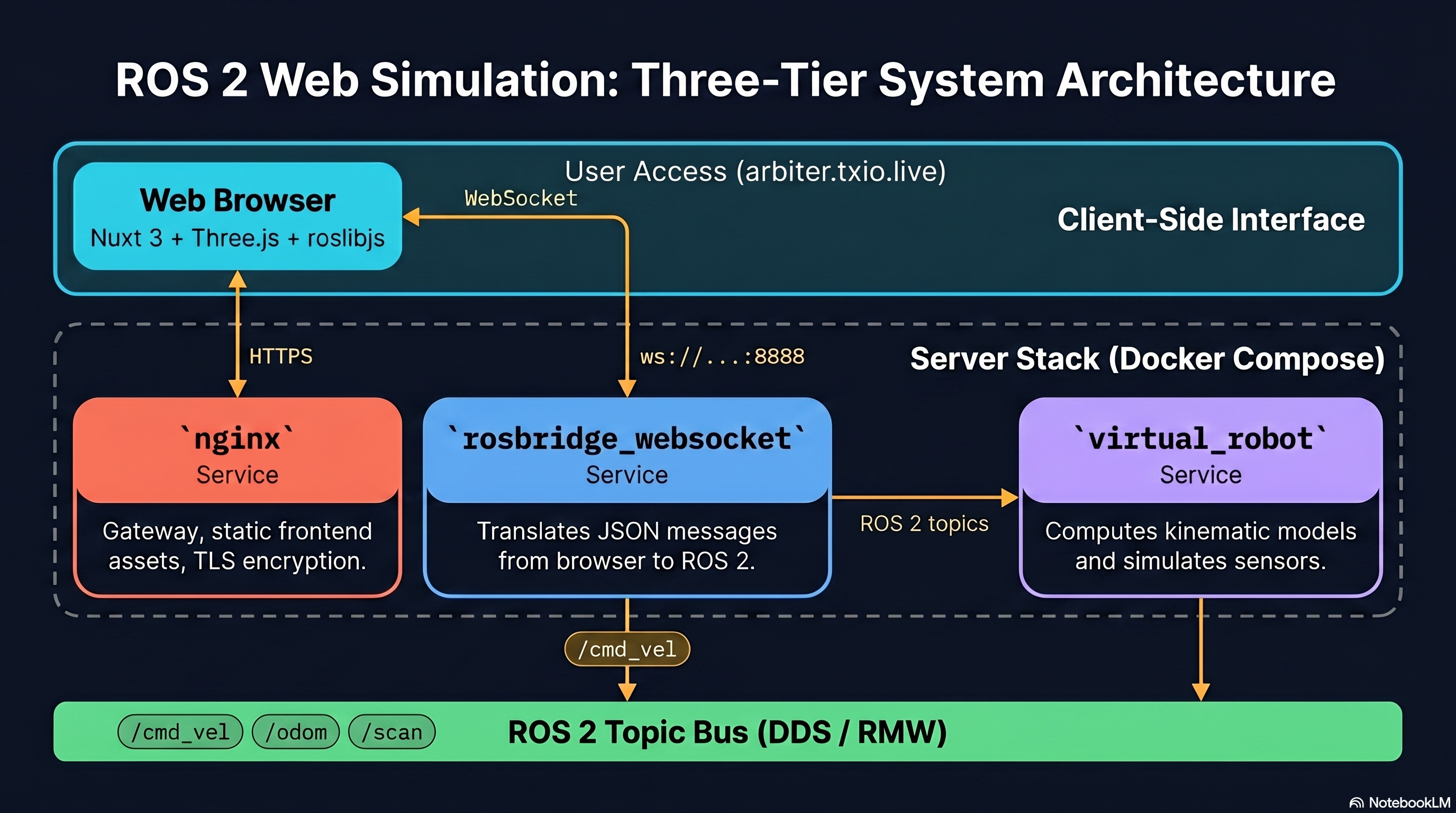
2.5.2 Platform Architecture

The simulation platform consists of four components orchestrated by Docker Compose. Each component runs in its own container, and the containers communicate through ROS 2 topics internally and WebSocket connections externally.

2.5.2.1 Docker Compose Orchestration

Docker Compose defines two primary services: ros2-web-bridge and web-interface. The ros2-web-bridge service contains the ROS 2 Humble runtime, the virtual robot node, and the rosbridge WebSocket server. The web-interface service contains an nginx web server that serves the HTML and JavaScript frontend to the student’s browser. Both services share a common Docker network so that the rosbridge server is accessible to the web server, and ports 9090 (WebSocket) and 8080 (HTTP) are exposed to the host network.

2.5.2.2 The Kinematic Model

The virtual robot implements a differential drive kinematic model. At each time step, the robot’s pose is updated using the velocity commands received on /cmd_vel. The discrete-time kinematic equations are:

x_{k} = x_{k - 1} + v * cos (θ_{k - 1}) * d t (1)

y_{k} = y_{k - 1} + v * sin (θ_{k - 1}) * d t (2)

θ_{k} = θ_{k - 1} + ω * d t (3)

where v is the linear velocity (from twist.linear.x), omega is the angular velocity (from twist.angular.z), dt is the time step (0.05 seconds at 20 Hz), and ( $x_{k}$ , $y_{k}$ , $θ_{k}$ ) is the robot’s pose at step k. These are the same kinematic equations derived in Module 2.2 for the unicycle model. The simulation applies them directly: it receives velocity commands and integrates them forward in time to produce the robot’s trajectory.

Default platform parameters. The constructor options for MobileRobotPhysics (at frontend/lib/Robot/MobileRobotPhysics.js) ship with the following defaults, reused across every page of the platform and by every assessment in this course:

Symbol	Value	Meaning
$m$	$2.0$ kg	chassis mass
$r$	$0.033$ m	wheel radius (not $0.05$ m)
$L$	$0.16$ m	wheelbase (distance between drive wheels)
$I$	$0.01$ kg m $^{2}$	moment of inertia about the vertical axis
$v_{m a x}$	$0.7$ m/s	linear-velocity limit enforced by $useROSBridge$
$ω_{m a x}$	$1.5$ rad/s	angular-velocity limit

These numbers match the Pi 4B hardware configuration in backend/config/pi4b_params.yaml, so a controller tuned against the virtual robot transfers to the physical platform without re-tuning. Assignment 1 derives $M (q) \overset{q}{¨} + C (q, \overset{q}{˙}) \overset{q}{˙} = B τ$ using exactly this parameter set; the Bonus Task perturbs $m$ and $I$ at runtime from /admin to stress payload sensitivity.

2.5.2.3 Rosbridge WebSocket Bridge

The rosbridge_server package provides a WebSocket interface to the ROS 2 middleware on port 9090. It translates between JSON messages sent over WebSocket and native ROS 2 messages. When a browser client publishes a JSON-encoded Twist message to the WebSocket, rosbridge deserializes it and publishes a native geometry_msgs/Twist message on the /cmd_vel topic. In the reverse direction, when the virtual robot publishes odometry or laser scan data, rosbridge serializes these messages to JSON and sends them to all connected WebSocket clients. This bridge is the critical link that allows browser-based JavaScript to interact with the ROS 2 ecosystem without any ROS 2 installation on the client side.

2.5.2.4 Nginx Web Server

The nginx container serves static HTML, CSS, and JavaScript files on port 8080. These files constitute the simulation frontend: a 2D visualization of the robot, its laser scan data, and the obstacle map, along with controls for sending velocity commands. The frontend uses the roslibjs JavaScript library to establish a WebSocket connection to the rosbridge server and communicate with ROS 2 topics.

2.5.2.5 Data Flow

The complete data flow for a velocity command is:

Browser (JavaScript) $\to$ WebSocket (port 9090) $\to$ rosbridge_server $\to$ /cmd_vel topic $\to$ virtual_robot.py $\to$ kinematic update $\to$ /odom, /scan, /tf topics $\to$ rosbridge_server $\to$ WebSocket $\to$ Browser (JavaScript)

This round-trip occurs at the simulation’s update rate of 20 Hz. The student sees the robot move in the browser visualization within one update cycle (50 ms) of sending a command.

2.5.3 The Virtual Robot Node

The virtual_robot.py node is the core of the simulation. It is a standard ROS 2 Python node that subscribes to velocity commands, integrates the kinematic model, and publishes sensor data.

2.5.3.1 Core Update Loop

The node runs a timer callback at 20 Hz that performs the kinematic integration and publishes all output data:

  // Core kinematic update in virtual_robot.py
  def update_robot_state(self):
      dt = 0.05  // 20 Hz update rate
      self.x += self.linear_vel * math.cos(self.theta) * dt
      self.y += self.linear_vel * math.sin(self.theta) * dt
      self.theta += self.angular_vel * dt
      self.publish_odometry()
      self.broadcast_transform()

The linear_vel and angular_vel values are set by the /cmd_vel subscriber callback whenever a new Twist message arrives. Between messages, the robot continues at its last commanded velocity, which matches the behavior of a real differential drive robot with a motor controller that maintains commanded speed.

2.5.3.2 Odometry Publishing

The node publishes nav_msgs/Odometry messages on the /odom topic at 20 Hz. Each message contains the robot’s position (x, y, z) in the pose.pose.position fields, the robot’s orientation as a quaternion in pose.pose.orientation (computed from theta using the standard conversion: w = cos(theta/2), z = sin(theta/2), x = y = 0), and the robot’s velocity in the twist.twist fields (linear.x = v, angular.z = omega). The odometry frame_id is "odom" and the child_frame_id is "base_link", following the ROS 2 REP 105 convention.

2.5.3.3 TF Broadcasting

The node broadcasts the transform from the "odom" frame to the "base_link" frame using a tf2 TransformBroadcaster. This transform encodes the same pose information as the odometry message but in the TF tree format that other ROS 2 nodes (such as rviz2 or navigation stacks) expect. The translation is (x, y, 0) and the rotation is the quaternion computed from theta. Broadcasting this transform ensures that any ROS 2 node that queries the relationship between odom and base_link receives the correct answer, whether the data comes from the simulation or a real robot’s wheel encoders.

2.5.3.4 LaserScan Simulation

The node publishes sensor_msgs/LaserScan messages on the /scan topic by performing ray-casting against a simple obstacle map. The obstacle map is defined as a list of line segments (walls) in the simulation’s coordinate frame. For each ray in the scan (typically 360 rays spanning 0 to 2*pi), the node computes the intersection of the ray originating from the robot’s current pose with each wall segment and reports the distance to the nearest intersection. If no wall is intersected within the maximum range, the ray returns the maximum range value.

The scan parameters match a typical low-cost LiDAR: angle_min = 0, angle_max = 2pi, angle_increment = 2pi/360, range_min = 0.12 m, range_max = 3.5 m, and scan_time = 0.1 s. These values are chosen to approximate the RPLIDAR A1 sensor used on the physical robot platform, ensuring that algorithms developed in simulation encounter the same field of view, resolution, and range limitations as they will on the real hardware.

2.5.4 Docker Deployment

The entire simulation platform is packaged as a Docker Compose project. This ensures that every student runs exactly the same software stack, regardless of their host operating system.

2.5.4.1 Docker Compose Structure

The docker-compose.yml file defines the two services, their build contexts, port mappings, and shared network:

  // docker-compose.yml structure
  services:
    ros2-web-bridge:
      build: ./ros2-bridge
      ports:
        - "9090:9090"
      // Runs rosbridge_server and virtual_robot.py
    web-interface:
      build: ./web-interface
      ports:
        - "8080:80"
      // Runs nginx serving the frontend

The ros2-bridge directory contains the Dockerfile that installs ROS 2 Humble, rosbridge_server, and the virtual_robot.py node. The web-interface directory contains the Dockerfile for nginx and the static frontend files.

2.5.4.2 Building and Launching

To build the containers and start the simulation:

docker-compose up -d

The -d flag runs the containers in detached mode (in the background). On the first run, Docker builds the images from the Dockerfiles, which may take several minutes. Subsequent launches use cached images and start within seconds.

2.5.4.3 Monitoring

To check that both services are running:

docker-compose ps

This lists the running containers, their status, and their port mappings. Both services should show "Up" status. To view the logs from the ROS 2 bridge service (useful for debugging topic connections):

docker-compose logs ros2-web-bridge

To follow the logs in real time:

docker-compose logs -f ros2-web-bridge

2.5.4.4 Stopping

To stop all containers:

docker-compose down

This stops and removes the containers but preserves the built images. The next docker-compose up -d will start fresh containers from the existing images.

2.5.5 Connecting from the Browser

The student interacts with the simulation through a JavaScript frontend that uses the roslibjs library to communicate with ROS 2 via WebSocket.

2.5.5.1 WebSocket Connection

The roslibjs library establishes a WebSocket connection to the rosbridge server:

  // Connect to ROS 2 via WebSocket
  const ros = new ROSLIB.Ros({ url: 'ws://[pi-ip]:9090' });

  // Connection status callbacks
  ros.on('connection', function() { console.log('Connected to ROS 2'); });
  ros.on('error', function(error) { console.log('Error: ', error); });
  ros.on('close', function() { console.log('Connection closed'); });

When running the simulation locally, the URL is ws://localhost:9090. When connecting to a simulation running on a Raspberry Pi, replace localhost with the Pi’s IP address.

2.5.5.2 Publishing Velocity Commands

To command the virtual robot, the frontend creates a Topic object for /cmd_vel and publishes Twist messages:

  // Create the /cmd_vel topic
  const cmdVel = new ROSLIB.Topic({
      ros: ros,
      name: '/cmd_vel',
      messageType: 'geometry_msgs/msg/Twist'
  });

  // Send velocity command
  cmdVel.publish(new ROSLIB.Message({
      linear: { x: 0.3, y: 0.0, z: 0.0 },
      angular: { x: 0.0, y: 0.0, z: 0.0 }
  }));

This publishes a forward velocity of 0.3 m/s with no rotation. To turn the robot, set angular.z to a nonzero value. For example, angular.z = 0.5 commands a left turn at 0.5 rad/s. The message structure is identical to what a ROS 2 Python or C++ node would publish, the only difference is the JSON encoding handled transparently by roslibjs and rosbridge.

2.5.5.3 Subscribing to Odometry

To display the robot’s position in the browser, the frontend subscribes to the /odom topic:

  // Subscribe to odometry
  const odomListener = new ROSLIB.Topic({
      ros: ros,
      name: '/odom',
      messageType: 'nav_msgs/msg/Odometry'
  });

odomListener.subscribe(function(message) {

co n s t \times co n s t y = m ess a g e . p ose . p ose . p os i t i o n . x; = m ess a g e . p ose . p ose . p os i t i o n . y;

      // Update browser display with robot position
  });

Each odometry message arrives at 20 Hz, providing smooth position updates for the visualization.

2.5.5.4 Subscribing to LaserScan

To visualize obstacles detected by the simulated LiDAR, the frontend subscribes to /scan:

  // Subscribe to laser scan
  const scanListener = new ROSLIB.Topic({
      ros: ros,
      name: '/scan',
      messageType: 'sensor_msgs/msg/LaserScan'
  });

scanListener.subscribe(function(message) {

co n s t r an g es = m ess a g e . r an g es; // A r r a y o f 360 d i s t an ce v a l u es

      // Draw scan points on the 2D visualization canvas
  });

The ranges array contains 360 distance values corresponding to angles from 0 to 2*pi. Each value represents the distance to the nearest obstacle along that ray. The frontend converts these polar coordinates to Cartesian coordinates relative to the robot’s position and renders them as points on the 2D canvas.

2.5.6 Sim-to-Real Transition

The primary design goal of the web-browser simulation platform is that code developed in simulation transfers to the real robot with zero modifications to the control logic.

2.5.6.1 Topic Compatibility

The simulation publishes and subscribes to the same topics as the physical robot:

/cmd_vel (geometry_msgs/Twist): Velocity commands consumed by the virtual robot in simulation and by the motor controller on the real robot
/odom (nav_msgs/Odometry): Pose and velocity feedback produced by the kinematic model in simulation and by wheel encoder integration on the real robot
/scan (sensor_msgs/LaserScan): LiDAR data produced by ray-casting in simulation and by the RPLIDAR A1 sensor on the real robot
/tf (tf2_msgs/TFMessage): Coordinate frame transforms produced by both the simulation and the real robot’s odometry node

Because the topic names and message types are identical, any ROS 2 node (or JavaScript client) that works in simulation will work on the real robot without code changes.

2.5.6.2 Deployment to Raspberry Pi 4B

The same docker-compose.yml used for simulation on a development machine can be deployed to a Raspberry Pi 4B. The Pi runs the Docker containers natively (ARM64 images are built for this purpose). The deployment process is: copy the docker-compose project to the Pi, run docker-compose up -d, and connect from a browser using the Pi’s IP address. When the physical robot hardware is connected, the virtual_robot.py node is replaced by the real robot’s driver nodes, but all other components (rosbridge, nginx, the frontend) remain the same.

2.5.6.3 The Only Change: WebSocket URL

In the JavaScript frontend, the transition from simulation to real robot requires changing a single line:

  // Simulation (running locally)
  const ros = new ROSLIB.Ros({ url: 'ws://localhost:9090' });

  // Real robot (running on Raspberry Pi at 192.168.1.100)
  const ros = new ROSLIB.Ros({ url: 'ws://192.168.1.100:9090' });

No other code changes are required. The topic names, message types, and interaction patterns are identical.

2.5.6.4 Validation

To verify that the simulation accurately represents the real robot’s behavior, students compare simulation odometry against real odometry for the same velocity command sequence. For a differential drive robot operating on a flat surface at low speeds (under 0.5 m/s), the kinematic model (Equations 1-3) is highly accurate. Discrepancies arise primarily from wheel slip, uneven terrain, and encoder noise, which are absent in the simulation. Understanding these discrepancies is itself a valuable learning exercise: it teaches students that simulation is an approximation and that robust control must account for model uncertainty.

2.5.7 Comparison with Gazebo (Reference Only)

This section provides context for students who encounter Gazebo in other courses or research settings.

Gazebo is a full-featured robotics simulator that includes a physics engine (ODE, Bullet, or DART), 3D rendering with realistic lighting and textures, sensor plugins for cameras, depth sensors, IMUs, and LiDAR, and support for contact physics, friction, and gravity. Gazebo is the standard simulator for ROS-based research and is used extensively in competitions such as the DARPA SubT Challenge. However, Gazebo requires a GPU for real-time 3D rendering, consumes several gigabytes of disk space for installation, demands significant CPU and RAM resources, and has a complex configuration process involving SDF/URDF models, world files, and plugin configurations.

The web-browser platform takes a fundamentally different approach. It uses a kinematic-only model (no physics engine), renders in 2D in the browser (no GPU required), consumes minimal CPU and RAM (runs on a Raspberry Pi), and requires zero client-side installation.

When to use Gazebo: Research requiring accurate contact physics (grasping, legged locomotion), applications needing 3D perception (camera-based object detection, depth-based navigation), and projects where photorealistic rendering is needed for training perception models.

When to use the web platform: Education where the learning objective is control and navigation algorithms rather than perception, deployment scenarios where the target hardware is resource-constrained, rapid prototyping where fast iteration is more valuable than physical accuracy, and situations where universal student access is a requirement.

For the differential drive mobile robot platform used in this course, the kinematic model is sufficiently accurate for all control and navigation tasks covered in Modules 2 through 5. The web-browser platform provides all the sensing and actuation interfaces needed while eliminating the installation and configuration burden that consumes valuable instructional time.

Integration: Theory to Practice

The web-browser simulation platform connects directly to the PID control framework from Module 2.4. The virtual robot subscribes to /cmd_vel and publishes /odom, forming the plant in the feedback control loop. The PID controller node (or JavaScript equivalent) reads the current pose from /odom, computes the error relative to the desired setpoint, evaluates the PID equation (Module 2.4, Equation 9), and publishes the resulting velocity command on /cmd_vel. The virtual robot receives this command, integrates the kinematic model (Equations 1-3), and publishes the updated pose. This closed loop runs continuously at the controller’s update rate (10 Hz for the PID node from Module 2.4) nested within the simulation’s 20 Hz update rate. Students can observe the feedback loop in real time through the browser visualization: commanding a heading setpoint and watching the robot rotate, overshoot (if the gains are too high), and settle to the desired heading. The simulation provides immediate visual feedback on the effect of tuning $K_{p}$ , $K_{i}$ , and $K_{d}$ , making abstract control theory tangible. Because the simulation and real robot share the same topic interface, a PID controller tuned in simulation can be deployed to the physical robot by changing only the WebSocket URL, and the student can compare the simulated response to the real response side by side.

Theoretical Design Choices

The kinematic-only simulation model is chosen deliberately over a full dynamic simulation. For a mobile robot operating at speeds below 1 m/s on a flat surface, the kinematic model (Equations 1-3) captures the dominant behavior: the robot goes where its velocity commands direct it, with negligible lag from inertia or wheel dynamics. Adding a dynamic model with mass, inertia, and friction would increase the simulation’s fidelity but would also increase its complexity and computational requirements without improving the educational outcomes for this course. The kinematic model is exact for an ideal differential drive robot, and the differences between it and the real robot’s behavior teach students about the gap between models and reality, which is itself a fundamental lesson in robotics.

Docker is chosen for deployment because it guarantees reproducibility. Every student runs exactly the same ROS 2 version, the same rosbridge configuration, and the same virtual robot code, regardless of their host operating system. This eliminates the "it works on my machine" problem that plagues robotics courses using native installations. Docker also simplifies deployment to the Raspberry Pi: the same Compose file works on both the development machine and the target hardware, ensuring that the simulation environment and the deployment environment are identical.

The WebSocket bridge architecture (rosbridge) is chosen over native ROS 2 client libraries in the browser because WebSocket is universally supported by all browsers without plugins or extensions. Native ROS 2 communication uses DDS (Data Distribution Service), which requires platform-specific binary libraries that cannot run in a browser. The rosbridge approach trades a small amount of latency (JSON serialization overhead) for universal accessibility, which is the correct trade-off for an educational platform where ease of access is paramount.