○Draft — not verified

Closed-loop PID block diagram with parallel proportional, integral, and derivative branches summing into the plant, with sensor feedback to the error junction — Canonical closed-loop PID: the error e(t) feeds parallel Kp, Ki∫, and Kd·d/dt branches whose sum u(t) drives the plant; sensor feedback closes the loop.

Theoretical Background: PID Control for Mobile Robots

Module 2 Theory: PID Control

2.3.1 Feedback Control Fundamentals

Control systems fall into two categories. An open-loop controller computes the control input based solely on the desired output, with no measurement of what the system actually does. A conveyor belt running at a fixed motor voltage is open-loop: if the load changes, the belt speed changes with no correction. A closed-loop (feedback) controller measures the actual output, compares it to the desired output, and adjusts the input to reduce the difference.

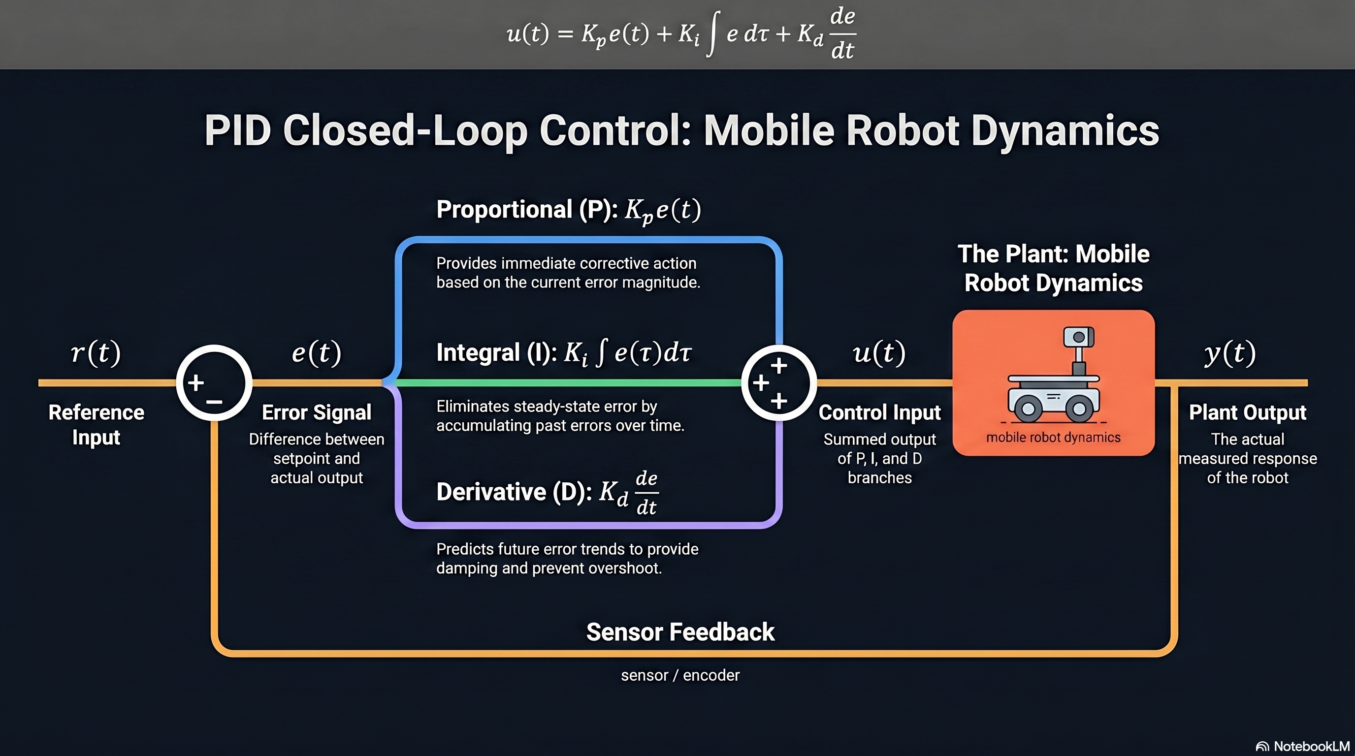
The Feedback Control Loop:

Reference $r (t)$ : The desired value (setpoint) that the system should track
Error $e (t)$ : The difference between what we want and what we have
Controller: Computes a control signal $u (t)$ based on the error
Plant: The physical system being controlled (the robot)
Output $y (t)$ : The measured response of the plant
Sensor: Measures $y (t)$ and feeds it back for comparison with $r (t)$

The signal flow is: Reference $\to$ Summing Junction $\to$ Controller $\to$ Plant $\to$ Output, with the sensor feeding the output back to the summing junction. The error signal is:

e (t) = r (t) - y (t) (1)

Why Feedback: Open-loop control fails when the plant model is inaccurate, disturbances act on the system, or parameters change over time. For mobile robots, all three conditions hold: the dynamics are nonlinear and coupled, the terrain introduces disturbances, and tire friction varies with surface conditions. Feedback is essential.

2.3.2 Proportional Control (P)

The simplest feedback controller applies a control effort proportional to the current error:

u (t) = K_{p} e (t) (2)

where $K_{p}$ is the proportional gain. When the error is large, the control effort is large. When the error is small, the control effort is small. When the error is zero, the control effort is zero.

Effect of $K_{p}$ : Increasing $K_{p}$ makes the system respond faster to errors, reduces steady-state error (but does not eliminate it), increases overshoot and oscillation, and can eventually cause instability if set too high. There is a fundamental trade-off: higher gain improves tracking but degrades stability.

Steady-State Error: For a type-0 system (no free integrators in the plant), proportional control alone cannot eliminate steady-state error for a step input. The steady-state error is:

e_{ss} = \frac{1}{1 + K _{p} G ( 0 )}

where $G (0)$ is the DC gain of the plant. Increasing $K_{p}$ reduces $e_{ss}$ but never drives it to zero.

Mobile Robot Heading Control: For a differential drive robot where the plant maps angular velocity to heading, proportional heading control takes the form:

ω = K_{p} (θ_{d} - θ) (3)

where $θ_{d}$ is the desired heading and $θ$ is the current heading. This controller commands the robot to turn faster when the heading error is large and slower as it approaches the target heading. In practice, the heading error should be wrapped to $[- π, π]$ to avoid discontinuities at the $\pm π$ boundary.

2.3.3 Integral Control (I)

Integral control applies effort proportional to the accumulated error over time:

u (t) = K_{i} \int_{0}^{t} e (τ) d τ (4)

where $K_{i}$ is the integral gain. The integral accumulates error: even a small persistent error will eventually produce a large control signal. This is the mechanism that eliminates steady-state error. If any error persists, the integral grows until the controller drives the error to zero.

Why Integral Action Works: Consider a system with proportional control that has a steady-state error of 0.1. The proportional term produces a constant control effort that is insufficient to close the gap. Adding integral action means this 0.1 error is continuously integrated, producing a control signal that grows over time until the additional effort eliminates the remaining error.

Integral Windup: When the actuator saturates (reaches its physical limit), the integral term continues to accumulate error even though the controller output cannot increase further. When the error eventually reverses sign, the integral must “unwind” before the controller responds, causing large overshoot and sluggish recovery.

Anti-Windup Strategies:

Clamping: Stop integrating when the controller output exceeds the actuator limits. The integral is frozen at its current value until the output returns within bounds.
Back-Calculation: When the actuator saturates, compute the difference between the desired and actual controller output and feed it back to reduce the integral term. This approach provides smoother transitions in and out of saturation.

For mobile robots, actuator limits are real: wheel motors have maximum angular velocities, and the /cmd_vel interface typically enforces velocity bounds.

2.3.4 Derivative Control (D)

Derivative control applies effort proportional to the rate of change of the error:

u (t) = K_{d} \frac{d e ( t )}{d t} (5)

where $K_{d}$ is the derivative gain. If the error is decreasing rapidly, the derivative term reduces the control effort, providing a braking effect that reduces overshoot. If the error is increasing, the derivative term adds effort to counteract the trend before the error becomes large.

Damping Effect: Derivative action is analogous to a viscous damper in a mechanical system. Without it, a proportional controller with high gain will oscillate. The derivative term predicts the future error trend from its current rate of change and acts preemptively.

Noise Amplification Problem: Differentiation amplifies high-frequency noise. If the error signal contains measurement noise at frequency $f$ , the derivative amplifies that noise by a factor proportional to $f$ . For a mobile robot using encoder-based odometry, quantization noise in the position estimate produces spikes in the derivative term.

Practical Filtered Derivative: In practice, the pure derivative is replaced by a filtered derivative using a first-order low-pass filter:

D (s) = \frac{K _{d} s}{1 + τ _{f} s}

where $τ_{f}$ is the filter time constant, typically chosen as $τ_{f} = K_{d} / (8 K_{p})$ to $K_{d} / (20 K_{p})$ . This limits the high-frequency gain to $K_{d} / τ_{f}$ rather than allowing it to grow without bound.

2.3.5 Combined PID Controller

The full PID controller combines all three actions:

u (t) = K_{p} e (t) + K_{i} \int_{0}^{t} e (τ) d τ + K_{d} \frac{d e ( t )}{d t} (6)

Each term serves a distinct role: proportional provides the primary corrective action based on current error, integral eliminates steady-state error by responding to accumulated past error, and derivative provides damping by responding to the error trend.

Transfer Function Form:

C (s) = K_{p} + \frac{K _{i}}{s} + K_{d} s (7)

This can be written in the standard form using integral time $T_{i} = K_{p} / K_{i}$ and derivative time $T_{d} = K_{d} / K_{p}$ :

C (s) = K_{p} (1 + \frac{1}{T _{i} s} + T_{d} s) (8)

Key Insight: $T_{i}$ determines how long the controller “remembers” past errors (smaller $T_{i}$ means faster integral action), and $T_{d}$ determines how far into the future the controller “predicts” (larger $T_{d}$ means stronger anticipation).

Discrete-Time Implementation: Digital controllers operate at a fixed sample rate. The continuous PID must be discretized for implementation. Using backward Euler integration for the integral and backward difference for the derivative:

u_{k} = K_{p} e_{k} + K_{i} Δ t j = 0 \sum k e_{j} + K_{d} \frac{e _{k} - e _{k - 1}}{Δ t} (9)

where $Δ t$ is the sample period and $e_{k} = e (k Δ t)$ . The integral is accumulated as a running sum, and the derivative is approximated by a first-order difference. This form is directly implementable in a ROS 2 control node.

2.3.6 PID Tuning Methods

Ziegler-Nichols Oscillation Method: This classical method requires no plant model. The procedure is: set $K_{i} = 0$ and $K_{d} = 0$ , increase $K_{p}$ from zero until the system exhibits sustained oscillations, record the ultimate gain $K_{u}$ (the $K_{p}$ value at sustained oscillation) and the ultimate period $T_{u}$ (the period of oscillation).

Ziegler-Nichols tuning rules:

P only: $K_{p} = 0.5 K_{u}$
PI: $K_{p} = 0.45 K_{u}$ , $T_{i} = T_{u} /1.2$
PID: $K_{p} = 0.6 K_{u}$ , $T_{i} = T_{u} /2$ , $T_{d} = T_{u} /8$

Important: Ziegler-Nichols tuning produces an aggressive response with approximately 25% overshoot. For mobile robots, this is often unacceptable (overshoot in heading control means the robot turns past its target). The Ziegler-Nichols values should be used as a starting point and then reduced.

Manual Tuning Heuristics: A systematic manual approach:

Step 1: Start with P only. Increase $K_{p}$ until the response is fast but oscillatory.
Step 2: Add D for damping. Increase $K_{d}$ until oscillations are suppressed. The system should now converge smoothly but may have steady-state error.
Step 3: Add I for steady-state accuracy. Increase $K_{i}$ slowly until the steady-state error is eliminated. Too much $K_{i}$ will reintroduce oscillations.

Practical Observation: Many mobile robot controllers use PD only (no integral term). The integral term is omitted when steady-state error is acceptable or when the controller is re-computed frequently enough (as in a path-following loop where new setpoints arrive faster than steady-state is reached).

2.3.7 PID for Mobile Robot Applications

Mobile robots require multiple PID loops operating simultaneously on different controlled variables.

Linear Velocity Control: Regulates the forward speed of the robot:

v = K_{p, v} e_{v} + K_{i, v} \int e_{v} d t + K_{d, v} \frac{d e _{v}}{d t} (10)

where $e_{v} = v_{d} - v_{actual}$ is the velocity error. This controller ensures the robot maintains the commanded speed despite terrain variations and load changes. The velocity is typically estimated from wheel encoder differences.

Heading Control: Regulates the orientation of the robot. A PD controller is often sufficient:

ω = K_{p, ω} e_{θ} + K_{d, ω} \frac{d e _{θ}}{d t} (11)

where $e_{θ} = θ_{d} - θ$ is the heading error. Integral action is usually omitted for heading control because the integrator can cause unwanted turning when the desired heading changes frequently, heading errors due to disturbances are transient and self-correcting in a navigation loop, and the navigation planner continuously updates $θ_{d}$ , preventing steady-state conditions.

Distance-to-Goal Control: For point-to-point navigation, the linear velocity can be modulated based on the distance to the goal:

v_{cmd} = K_{p, d} d_{goal}

where $d_{goal} = (x_{g} - x)^{2} + (y_{g} - y)^{2}$ is the Euclidean distance to the goal position. This naturally slows the robot as it approaches the target. The desired heading is computed as $θ_{d} = atan2 (y_{g} - y, x_{g} - x)$ , which is then tracked by the heading controller (Equation 11).

Wall Following Controller: Maintains a desired distance $d_{ref}$ from a wall using LiDAR range measurements. The error is $e_{wall} = d_{ref} - d_{measured}$ , and a PD controller commands angular velocity to steer toward or away from the wall. The derivative term is critical here to prevent oscillatory zig-zag behavior.

Line Following Controller: Tracks a line on the ground (or a virtual path in the map). The cross-track error $e_{ct}$ is the perpendicular distance from the robot to the line. A PD controller on $e_{ct}$ commands angular velocity corrections:

ω = K_{p, ct} e_{ct} + K_{d, ct} \frac{d e _{ct}}{d t}

For curved paths, a feedforward term based on the path curvature improves tracking performance.

2.3.8 Limitations of PID for Robotics

PID control is a linear control technique applied to a fundamentally nonlinear system. This mismatch has several consequences.

Linearity Assumption: PID gains are tuned at a specific operating point. A mobile robot operating at different speeds, on different surfaces, or carrying different payloads may require different gains. A PID controller tuned for straight-line driving at 0.5 m/s may perform poorly during tight turns or at 2.0 m/s.

No Model Knowledge: PID uses only the error signal and ignores the known physics of the robot. Model-based controllers such as computed torque control (for manipulators) or feedback linearization (for mobile robots) exploit the dynamic model to cancel nonlinearities, achieving better performance with less tuning effort.

Cross-Coupling Ignored: Independent PID loops on linear velocity and angular velocity ignore the coupling between them. In a differential drive robot, commanding a high angular velocity while trying to maintain forward speed requires coordinated wheel commands. Separate PID loops do not account for this interaction.

When PID Is Sufficient: PID works well when the system operates near a single operating point, the plant is approximately linear over the operating range, sample rates are fast relative to the system dynamics, and simplicity is more valuable than optimality. For most educational and research mobile robots operating at low speeds on flat surfaces, PID is entirely adequate.

When to Upgrade: Consider more advanced controllers when the robot operates over a wide range of speeds and configurations (gain scheduling or adaptive control), precise trajectory tracking is required with known dynamics (feedback linearization), constraints on states or inputs must be respected (model predictive control), or the system has significant nonlinearities that cause PID to perform poorly across operating conditions.

Script Implementation:

# PID controller class for mobile robot
        # Discrete-time implementation at 10 Hz
        
        class PIDController:
        def __init__(self, kp, ki, kd, dt=0.1):
        self.kp = kp
        self.ki = ki
        self.kd = kd
        self.dt = dt
        self.integral = 0.0
        self.prev_error = 0.0
        
        def compute(self, error):
        self.integral += error * self.dt
        derivative = (error - self.prev_error) / self.dt
        output = self.kp * error + self.ki * self.integral + self.kd * derivative
        self.prev_error = error
        return output
        
        # Usage for heading control
        heading_pid = PIDController(kp=2.0, ki=0.1, kd=0.5)
        angular_vel = heading_pid.compute(theta_desired - theta_current)
        
        # Usage in a ROS 2 control loop
        # The timer callback fires at 10 Hz
        # Each cycle: read sensors, compute error, call pid.compute(), publish /cmd_vel

Integration: Theory to Practice

The discrete PID equation (Equation 9) maps directly to a ROS 2 timer callback running at 10 Hz: each cycle reads the current state from odometry or sensor topics, computes the error relative to the setpoint, evaluates the PID equation, and publishes the result as a geometry_msgs/Twist message on /cmd_vel. The linear velocity output from the velocity PID (Equation 10) becomes twist.linear.x, and the angular velocity from the heading PID (Equation 11) becomes twist.angular.z. These two values are the inputs to the unicycle model from Module 2.2: $v$ drives forward motion and $ω$ drives rotation. Anti-windup clamping should match the velocity limits configured in the robot’s motor controller or the nav2 velocity smoother. The 10 Hz control rate ( $Δ t = 0.1$ s) is adequate for slow mobile robots (under 1 m/s) but should be increased to 20–50 Hz for faster platforms or when derivative action is used, since the finite-difference derivative approximation degrades at low sample rates.

Theoretical Design Choices

PID is chosen as the default starting controller for mobile robots because it requires no plant model, has only three parameters to tune, and provides acceptable performance across a wide range of operating conditions. The proportional-derivative structure (Equations 3 and 11) is preferred for heading control because integral action introduces phase lag that degrades transient response when setpoints change frequently, as occurs in path following. The Ziegler-Nichols method is presented as a systematic starting point, but its aggressive tuning (25% overshoot) is rarely appropriate for mobile robots where overshoot corresponds to physical deviation from the desired path. Manual tuning starting from P-only and adding D then I gives the engineer direct insight into each term’s contribution. When performance requirements exceed what PID can deliver, the natural progression is to gain scheduling (PID with operating-point-dependent gains), feedback linearization (cancels known nonlinearities, reduces the system to a linear one that PID can control optimally), and model predictive control (handles constraints and preview information, but requires an accurate model and significant computation). The PID framework remains valuable even when these advanced methods are used, because the inner velocity loops on most commercial mobile robot platforms are PID controllers running on dedicated motor driver hardware.