○Draft — not verified

Gazebo + ROS 2 simulation pipeline from URDF through physics engine and simulated sensors, bridged via ros_gz_bridge into SLAM/Nav2 and controller nodes — Simulation stack: URDF/Xacro feeds Gazebo's physics engine, simulated sensors publish through ros_gz_bridge onto ROS 2 topics consumed by SLAM, Nav2, and controllers.

Theoretical Background: Simulation of Dynamic Models

Module 2 Theory: Gazebo Simulation, URDF, and Sensor Modeling

2.3.1 Gazebo Simulation Environment

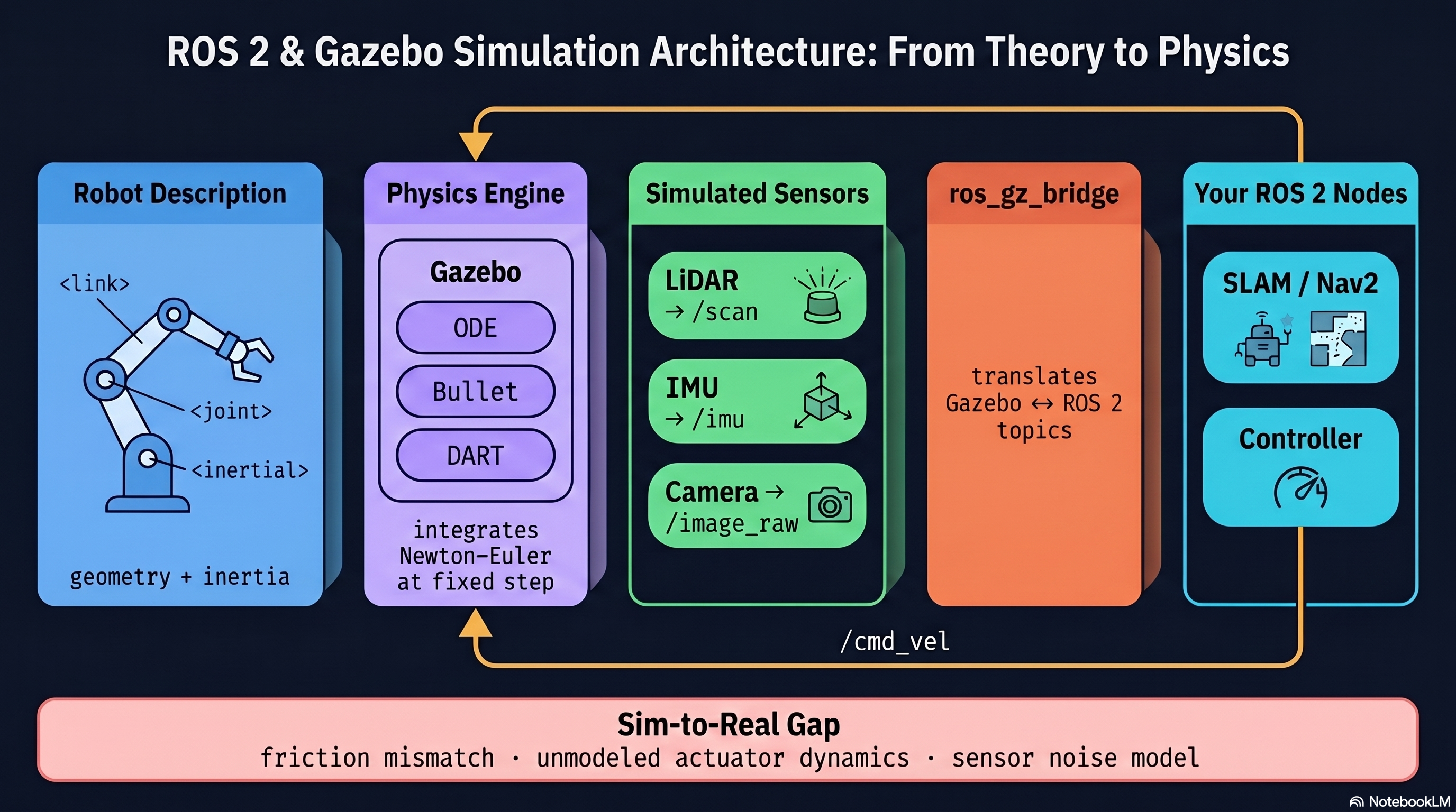
Gazebo is the primary physics simulator used with ROS 2 for robotics research. It provides rigid body dynamics, sensor simulation (LiDAR, cameras, IMUs, GPS), actuator models, environment modeling, and a plugin architecture for custom behavior.

Architecture: Gazebo runs two processes. gzserver executes the physics engine, sensor generation, and world simulation. gzclient provides the 3D graphical interface. Communication with ROS 2 occurs through the ros_gz_bridge package.

Launching Gazebo with ROS 2:

// Launch Gazebo with a world file
ros2 launch ros_gz_sim gz_sim.launch.py world_sdf_file:=my_world.sdf

// Bridge Gazebo topics to ROS 2
ros2 run ros_gz_bridge parameter_bridge /cmd_vel@geometry_msgs/msg/Twist@gz.msgs.Twist

2.3.2 Physics Engines in Robotics Simulation

Several physics engines are available, each with different trade-offs:

ODE (Open Dynamics Engine): Impulse-based, fast, good accuracy. Standard for general robotics.
Bullet: Impulse/constraint hybrid, fast. Common in gaming and robotics.
DART: Constraint-based, high accuracy, medium speed. Preferred for research and manipulation.
Simbody: Multibody dynamics, high accuracy, medium speed. Used in biomechanics.

Key Physics Parameters:

Step size (dt): Time between physics updates. Typical value is 0.001 s (1 kHz) for accurate dynamics.

Real-time factor (RTF): Ratio of simulation time to wall-clock time:

R T F = \frac{s i m _{t} im e _{e l a p se d}}{r e a l _{t} im e _{e l a p se d}} (1)

RTF = 1.0: Real-time simulation

$RTF > 1.0$ : Faster than real-time.

$RTF < 1.0$ : Slower than real-time.

Solver iterations: Number of constraint solver iterations per step. More iterations yield more accurate contact resolution. Typical range is 50-100 for stable simulation.

2.3.3 Contact Modeling

The spring-damper contact model computes normal forces at collision boundaries:

F_{contact} = k_{p} * p e n e t r a t i o n - k_{d} * v_{penetration} (2)

where $k_{p}$ is contact stiffness (position error gain), $k_{d}$ is contact damping (velocity error gain), and penetration is the depth of overlap between colliding bodies.

Practical Note: Setting $k_{p}$ too high causes numerical instability; setting it too low allows excessive interpenetration. Typical values for mobile robots on hard ground are $k_{p}$ = 10^5 to 10^7 N/m.

2.3.4 URDF Robot Description

URDF (Unified Robot Description Format) is the standard XML format for describing robots in ROS. A URDF model consists of links (rigid bodies) connected by joints.

Minimal Differential Drive Robot:

// URDF structure for a differential drive robot
<robot name="differential_drive_robot">

  // Base link with visual, collision, and inertial properties
  <link name="base_link">
    <visual>
      <geometry>
        <box size="0.3 0.2 0.1"/>
      </geometry>
      <material name="blue">
        <color rgba="0 0 0.8 1"/>
      </material>
    </visual>
    <collision>
      <geometry>
        <box size="0.3 0.2 0.1"/>
      </geometry>
    </collision>
    <inertial>
      <mass value="5.0"/>
      <inertia ixx="0.0208" ixy="0" ixz="0"
               iyy="0.0458" iyz="0" izz="0.0542"/>
    </inertial>
  </link>

  // Right wheel link
  <link name="right_wheel">
    <visual>
      <geometry>
        <cylinder radius="0.05" length="0.02"/>
      </geometry>
    </visual>
    <collision>
      <geometry>
        <cylinder radius="0.05" length="0.02"/>
      </geometry>
    </collision>
    <inertial>
      <mass value="0.5"/>
      <inertia ixx="0.0003" ixy="0" ixz="0"
               iyy="0.0003" iyz="0" izz="0.000625"/>
    </inertial>
  </link>

  // Continuous joint connecting wheel to chassis
  <joint name="right_wheel_joint" type="continuous">
    <parent link="base_link"/>
    <child link="right_wheel"/>
    <origin xyz="0 -0.11 -0.025" rpy="-1.5708 0 0"/>
    <axis xyz="0 0 1"/>
  </joint>
</robot>

2.3.5 Inertia Calculation for URDF

Every link in URDF requires an inertial element. The inertia tensor values must be computed correctly for accurate dynamic simulation.

Box (chassis) with mass m, dimensions d x w x h:

I_{xx} = (\frac{1}{12}) m (w^{2} + h^{2}) (3)

I_{y y} = (\frac{1}{12}) m (d^{2} + h^{2}) (4)

I_{z z} = (\frac{1}{12}) m (d^{2} + w^{2}) (5)

Cylinder (wheel) with mass m, radius r, length l:

I_{xx} = I_{y y} = (\frac{1}{12}) m (3 r^{2} + l^{2}) (6)

I_{z z} = (\frac{1}{2}) m r^{2} (7)

Key Requirement: If inertia values are omitted or set to zero, Gazebo will treat the link as having no mass, leading to simulation instability or the link being ignored by the physics engine.

2.3.6 Xacro for Parameterized Models

Xacro (XML Macros) allows parameterized, reusable robot descriptions. Parameters are defined once and referenced throughout the file, and macros encapsulate repeated structures like wheels.

Parameterized Wheel Macro:

// Xacro file with parameters and a wheel macro
<robot xmlns:xacro="http://www.ros.org/wiki/xacro" name="mobile_robot">

  // Define robot parameters once
  <xacro:property name="chassis_mass" value="5.0"/>
  <xacro:property name="wheel_radius" value="0.05"/>
  <xacro:property name="wheel_width" value="0.02"/>
  <xacro:property name="wheel_mass" value="0.5"/>
  <xacro:property name="wheelbase" value="0.22"/>

  // Wheel macro: reusable for left and right
  <xacro:macro name="wheel" params="prefix y_offset">
    <link name="${prefix}_wheel">
      <visual>
        <geometry>
          <cylinder radius="�PROTECT0�{wheel_width}"/>
        </geometry>
      </visual>
      <collision>
        <geometry>
          <cylinder radius="�PROTECT1�{wheel_width}"/>
        </geometry>
      </collision>
      <inertial>
        <mass value="${wheel_mass}"/>
        <inertia ixx="${(1.0/12.0)*wheel_mass*(3*wheel_radius*wheel_radius + wheel_width*wheel_width)}"
                 ixy="0" ixz="0"
                 iyy="${(1.0/12.0)*wheel_mass*(3*wheel_radius*wheel_radius + wheel_width*wheel_width)}"
                 iyz="0"
                 izz="${0.5*wheel_mass*wheel_radius*wheel_radius}"/>
      </inertial>
    </link>
    <joint name="${prefix}_wheel_joint" type="continuous">
      <parent link="base_link"/>
      <child link="${prefix}_wheel"/>
      <origin xyz="0 ${y_offset} -0.025" rpy="-1.5708 0 0"/>
      <axis xyz="0 0 1"/>
    </joint>
  </xacro:macro>

  // Instantiate both wheels from the macro
  <xacro:wheel prefix="right" y_offset="${-wheelbase/2}"/>
  <xacro:wheel prefix="left" y_offset="${wheelbase/2}"/>
</robot>

2.3.7 Sensor Simulation

LiDAR Sensor:

Gazebo simulates LiDAR by ray-casting in the physics world. The sensor definition specifies angular range, resolution, update rate, and range limits.

// LiDAR sensor definition in Gazebo SDF
<sensor name="lidar" type="gpu_lidar">
  <pose>0 0 0.15 0 0 0</pose>
  <topic>scan</topic>
  <update_rate>10</update_rate>
  <lidar>
    <scan>
      <horizontal>
        <samples>360</samples>
        <resolution>1</resolution>
        <min_angle>-3.14159</min_angle>
        <max_angle>3.14159</max_angle>
      </horizontal>
    </scan>
    <range>
      <min>0.12</min>
      <max>10.0</max>
    </range>
  </lidar>
</sensor>

IMU Sensor:

The IMU provides angular velocity and linear acceleration measurements. Realistic noise models are added to match physical sensor behavior.

// IMU sensor with Gaussian noise
<sensor name="imu" type="imu">
  <always_on>true</always_on>
  <update_rate>100</update_rate>
  <imu>
    <angular_velocity>
      <x><noise type="gaussian"><mean>0</mean><stddev>0.01</stddev></noise></x>
      <y><noise type="gaussian"><mean>0</mean><stddev>0.01</stddev></noise></y>
      <z><noise type="gaussian"><mean>0</mean><stddev>0.01</stddev></noise></z>
    </angular_velocity>
    <linear_acceleration>
      <x><noise type="gaussian"><mean>0</mean><stddev>0.1</stddev></noise></x>
      <y><noise type="gaussian"><mean>0</mean><stddev>0.1</stddev></noise></y>
      <z><noise type="gaussian"><mean>0</mean><stddev>0.1</stddev></noise></z>
    </linear_acceleration>
  </imu>
</sensor>

2.3.8 Differential Drive Controller Plugin

The gz-sim-diff-drive-system plugin converts cmd_vel twist messages into wheel joint commands, applying the kinematic model internally.

// Differential drive plugin configuration
<plugin filename="gz-sim-diff-drive-system"
        name="gz::sim::systems::DiffDrive">
  <left_joint>left_wheel_joint</left_joint>
  <right_joint>right_wheel_joint</right_joint>
  <wheel_separation>0.22</wheel_separation>
  <wheel_radius>0.05</wheel_radius>
  <max_linear_acceleration>1.0</max_linear_acceleration>
  <max_angular_acceleration>2.0</max_angular_acceleration>
  <topic>cmd_vel</topic>
  <odom_topic>odom</odom_topic>
</plugin>

2.3.9 Validating Simulation Against Real Systems

Simulation is only useful if it approximates real-world behavior. Validation follows a systematic methodology:

Parameter identification: Measure physical parameters (mass, inertia, friction coefficients) from the real robot
Open-loop comparison: Apply identical inputs to both the real robot and simulation, compare trajectories
Frequency response: Compare dynamic response characteristics across a range of input frequencies
Statistical analysis: Compute RMSE between simulated and real trajectories

Root Mean Square Error:

R M S E = sqrt ((\frac{1}{N}) i = 1 \sum N (x_{sim, i} - x_{real, i})^{2}) (8)

Common Sources of Sim-to-Real Gap:

Friction modeling: Affects steady-state accuracy. Mitigated by system identification.
Sensor noise: Affects perception performance. Mitigated by adding realistic noise models.
Motor dynamics: Affects transient response. Mitigated by including actuator models.
Contact modeling: Affects ground interaction. Mitigated by tuning contact parameters.
Unmodeled dynamics: Affects overall accuracy. Mitigated by domain randomization.

Domain Randomization:

This technique bridges the sim-to-real gap by randomizing simulation parameters during training:

// Randomize parameters to improve transfer to real hardware
friction_mu = random.uniform(0.3, 0.8)       // Range of surface friction
mass_scale = random.uniform(0.9, 1.1)        // +/- 10% mass variation
sensor_noise = random.gauss(0, 0.02)          // Gaussian sensor noise

2.3.10 Building and Launching a Simulated Robot

The workflow for creating a simulated robot in ROS 2 follows a standard sequence.

Step 1 – Create a ROS 2 package:

// Create workspace and package
mkdir -p ~/ros2_ws/src
cd ~/ros2_ws/src
ros2 pkg create --build-type ament_cmake my_robot_description

Step 2 – Create the URDF/Xacro file in my_robot_description/urdf/

Step 3 – Create a launch file:

// launch/gazebo.launch.py
// This Python launch file starts Gazebo and spawns the robot
def generate_launch_description():
    pkg_dir = get_package_share_directory('my_robot_description')
    return LaunchDescription([
        IncludeLaunchDescription(
            PythonLaunchDescriptionSource(
                os.path.join(get_package_share_directory('ros_gz_sim'),
                             'launch', 'gz_sim.launch.py')
            ),
            launch_arguments={'gz_args': '-r empty.sdf'}.items()
        ),
        Node(
            package='ros_gz_sim',
            executable='create',
            arguments=['-topic', 'robot_description', '-name', 'my_robot'],
            output='screen'
        ),
    ])

Step 4 – Build and launch:

// Build the workspace and launch simulation
cd ~/ros2_ws
colcon build
source install/setup.bash
ros2 launch my_robot_description gazebo.launch.py

Step 5 – Send velocity commands:

// Command the robot to drive forward at 0.5 m/s
ros2 topic pub /cmd_vel geometry_msgs/msg/Twist "{linear: {x: 0.5}, angular: {z: 0.0}}"

Integration: Theory to Practice

The dynamic model derived in Module 2.2 (Equations 17-18) determines the inertial and mass values entered into the URDF. When Gazebo loads the URDF, it constructs the mass matrix M and applies the physics engine’s contact and friction models to simulate wheel-ground interaction. The sensor noise parameters in the IMU and LiDAR definitions create the realistic measurement conditions that perception algorithms (Modules 5-6) must handle. The differential drive plugin implements the kinematic mapping from cmd_vel to wheel velocities, closing the loop between the navigation stack’s velocity commands and the simulated wheel joints. Validation against real hardware (RMSE analysis) determines whether the simulation fidelity is sufficient for controller development before deploying to the physical robot.

Theoretical Design Choices

URDF was chosen as the robot description format because it is the ROS ecosystem standard and directly consumed by both Gazebo and RViz2, avoiding format conversion errors. The spring-damper contact model (Equation 2) is preferred over impulse-based contact because it provides continuous forces that are easier for fixed-step integrators to handle, though it requires careful tuning of stiffness and damping parameters. Gaussian noise models for sensors are chosen because they match the first-order statistics of real sensor noise and are parameterized by only two values (mean and standard deviation) that can be measured from datasheets. Domain randomization is included as a validation technique because it addresses the fundamental limitation that no single set of simulation parameters perfectly matches reality – by training controllers across a distribution of parameters, robustness to modeling errors is built into the system rather than relying on perfect identification.