Theoretical Background: Robot Dynamics

Module 2 Theory: Lagrange Equations

2.1 Energy Methods vs. Force Methods

Classical mechanics provides two equivalent formulations for deriving equations of motion. The Newtonian approach requires explicit computation of all forces, including constraint forces at joints, making it cumbersome for multi-body robotic systems. The Lagrangian approach works with scalar energy quantities and eliminates constraint forces entirely, producing equations of motion directly in generalized coordinates.

Key Advantage: For an n-DOF serial robot, the Lagrangian method yields n second-order differential equations without ever computing internal joint reaction forces.

2.2 Kinetic and Potential Energy

Kinetic Energy of a rigid body combines translational and rotational contributions:

where m is the body mass, v is the linear velocity of the center of mass, omega is the angular velocity, and I is the inertia tensor about the center of mass.

For a system of n rigid bodies:

Potential Energy (gravitational):

where $r_i$ is the position of the center of mass of body i and g is the gravitational acceleration vector.

2.3 Generalized Coordinates

Generalized coordinates $q=[q_1,q_2,\dots ,q_n{]}^T$ are a minimal set of independent variables that completely describe the configuration of a mechanical system. For a serial robot manipulator with $n$ joints, each revolute joint contributes an angle $q_i={\theta }_i$ and each prismatic joint contributes a displacement $q_i=d_i$.

Example – 2-DOF Planar Robot:

End-effector position:

2.3.1 Holonomic vs. Nonholonomic Constraints

Holonomic constraints can be expressed as f(q, t) = 0 and reduce the number of independent coordinates. Nonholonomic constraints involve velocities and cannot be integrated into position-level equations. They do not reduce the configuration space dimension.

Example: The no-lateral-slip constraint for a differential drive robot is nonholonomic:

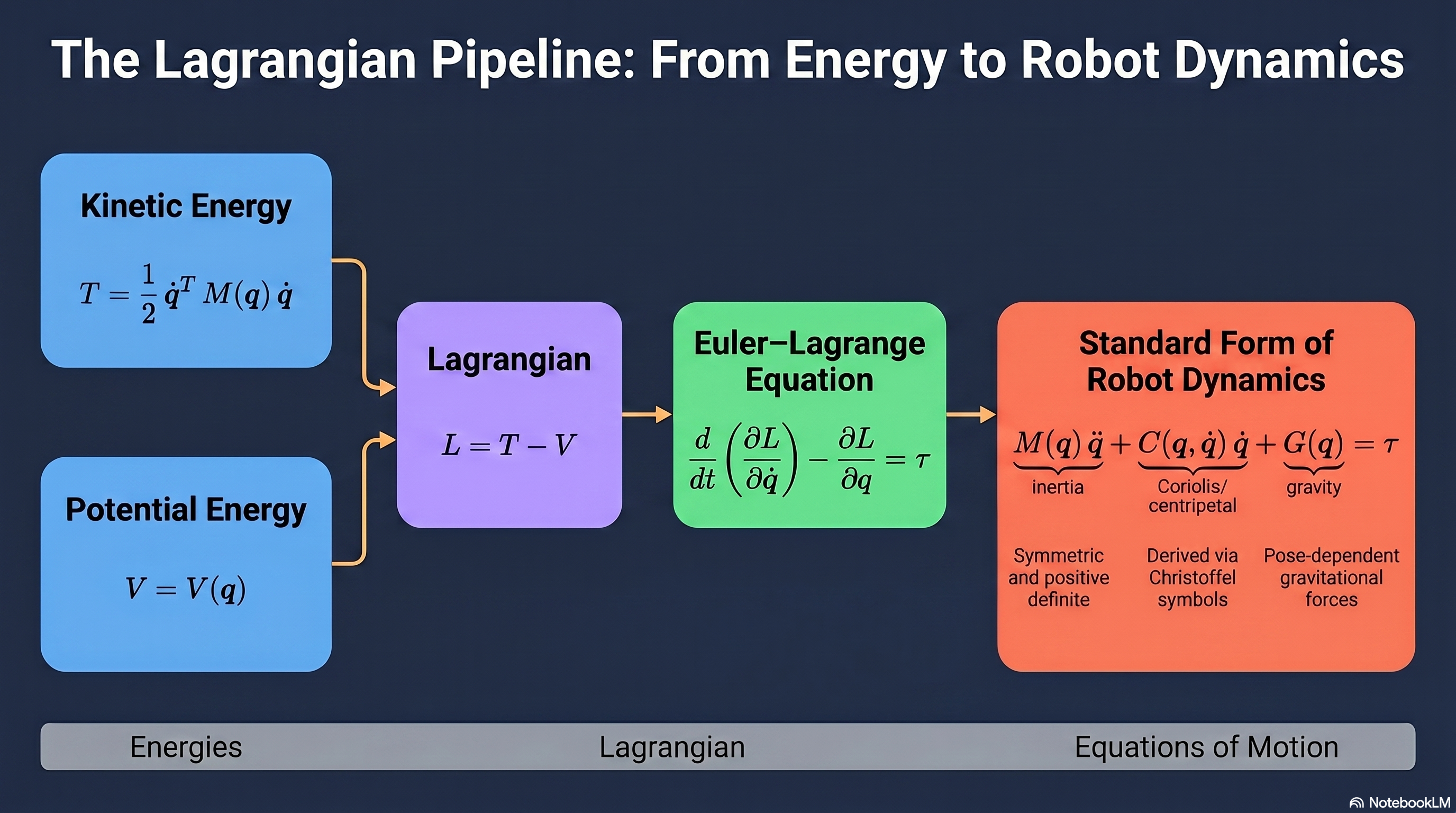
2.4 The Lagrangian and Euler-Lagrange Equations

The Lagrangian is defined as:

Hamilton’s Principle states that the actual motion minimizes the action integral:

Applying the calculus of variations (delta S = 0) yields the Euler-Lagrange equations:

for i = 1, 2, ..., n, where ${\tau }_i$ is the generalized force applied at joint i.

Since V does not depend on q_dot, this expands to:

2.5 Standard Form of Robot Dynamics

Applying the Euler-Lagrange equations to a robot manipulator yields:

M(q): n x n inertia (mass) matrix – symmetric, positive definite

C(q, q_dot): n x n Coriolis and centrifugal matrix

g(q): n x 1 gravity vector

tau: n x 1 joint torques/forces

2.5.1 Inertia Matrix Properties

The elements of M(q) are computed as:

Symmetric: $M_{ij}=M_{ji}$ for all $i,j$.

Positive definite: $x^{T}Mx>0$ for all $x\ne 0$.

Configuration dependent: $M$ changes with robot pose.

Bounded: ${\lambda }_{\min }I⪯M(q)⪯{\lambda }_{\max }I$.

2.5.2 Christoffel Symbols and the Coriolis Matrix

The Coriolis matrix elements are computed from Christoffel symbols of the first kind:

Skew-Symmetry Property:

Key Implication: This property is fundamental for proving stability of robot controllers via Lyapunov analysis, since x^T N x = 0 for all x.

2.6 Worked Example: 2-DOF Planar Manipulator

Consider a 2-link planar robot with link lengths $l_1$, $l_2$, masses $m_1$, $m_2$ concentrated at link ends, and joint angles ${\theta }_1$, ${\theta }_2$.

Step 1 – Kinetic Energy:

Velocity of mass 1:

Velocity of mass 2:

Total kinetic energy:

Step 2 – Potential Energy:

Step 3 – Lagrangian: L = T - V

Step 4 – Apply Euler-Lagrange Equations:

After differentiation, the resulting matrices are:

Inertia Matrix:

Coriolis Matrix:

Gravity Vector:

2.7 Lagrangian vs. Newton-Euler: When to Use Each

Lagrangian method: Best suited for deriving closed-form symbolic equations used in control design, stability analysis, and system identification. Computational complexity is O(n^4) symbolically.

Newton-Euler recursive method: Best suited for real-time torque computation, simulation, and inverse dynamics. Computational complexity is O(n) using the recursive formulation.

Practical Guideline: Use Lagrange to derive the structure of M, C, and g for controller design. Use Newton-Euler for online computation within the controller itself.

Integration: Theory to Practice

The standard form M(q) q_ddot + C(q, q_dot) q_dot + g(q) = tau is the foundation for all model-based robot control. In a ROS 2 implementation, the M, C, and g matrices are computed at each control cycle from joint encoder readings. The computed torque method inverts this equation to determine the feedforward torques needed for a desired trajectory, while the skew-symmetry property of N = M_dot - 2C guarantees passivity, which is exploited by adaptive and robust controllers. When transitioning from manipulators to mobile robots (Module 2.2), the same Lagrangian framework applies but must incorporate nonholonomic constraints via Lagrange multipliers.

Theoretical Design Choices

The choice of Lagrangian over Newtonian mechanics for robotics is driven by the elimination of internal constraint forces. For a 6-DOF manipulator, Newton-Euler requires computing forces at every joint just to cancel them later, whereas the Lagrangian approach works entirely in joint space. The use of Christoffel symbols to construct C(q, q_dot) rather than direct differentiation ensures the skew-symmetry property of M_dot - 2C is preserved, which is not guaranteed by arbitrary factorizations of the Coriolis terms. The positive definiteness of M(q) ensures that the dynamic equations are always well-posed and invertible, a property that control designers rely on when implementing computed torque or impedance control strategies.